dplyr filter(): Filter/Select Rows based on conditions

dplyr, R package that is at core of tidyverse suite of packages, provides a great set of tools to manipulate datasets in the tabular form. dplyr has a set of useful functions for “data munging”, including select(), mutate(), summarise(), and arrange() and filter().

And in this tidyverse tutorial, we will learn how to use dplyr’s filter() function to select or filter rows from a data frame with multiple examples. First, we will start with how to select rows of a dataframe based on a value of a single column or variable. And then we will learn how select rows of a dataframe using values from multiple variables or columns.

Let us get started by loading tidyverse, suite of R packges from RStudio.

library("tidyverse")

We will load Penguins data directly from cmdlinetips.com‘s github page.

path2data <- "https://raw.githubusercontent.com/cmdlinetips/data/master/palmer_penguins.csv"
penguins<- readr::read_csv(path2data)

Penguins data look like this

head(penguins)
## # A tibble: 6 x 7
##   species island bill_length_mm bill_depth_mm flipper_length_… body_mass_g sex  
##   <chr>   <chr>           <dbl>         <dbl>            <dbl>       <dbl> <chr>
## 1 Adelie  Torge…           39.1          18.7              181        3750 male 
## 2 Adelie  Torge…           39.5          17.4              186        3800 fema…
## 3 Adelie  Torge…           40.3          18                195        3250 fema…
## 4 Adelie  Torge…           NA            NA                 NA          NA <NA> 
## 5 Adelie  Torge…           36.7          19.3              193        3450 fema…
## 6 Adelie  Torge…           39.3          20.6              190        3650 male

Let us subset Penguins data by filtering rows based on one or more conditions.

How to filter rows based on values of a single column in R?

Let us learn how to filter data frame based on a value of a single column. In this example, we want to subset the data such that we select rows whose “sex” column value is “fename”.

penguins %>% 
  filter(sex=="female")

This gives us a new dataframe , a tibble, containing rows with sex column value “female”column.

## # A tibble: 165 x 7
##    species island bill_length_mm bill_depth_mm flipper_length_… body_mass_g
##    <chr>   <chr>           <dbl>         <dbl>            <dbl>       <dbl>
##  1 Adelie  Torge…           39.5          17.4              186        3800
##  2 Adelie  Torge…           40.3          18                195        3250
##  3 Adelie  Torge…           36.7          19.3              193        3450
##  4 Adelie  Torge…           38.9          17.8              181        3625
##  5 Adelie  Torge…           41.1          17.6              182        3200
##  6 Adelie  Torge…           36.6          17.8              185        3700
##  7 Adelie  Torge…           38.7          19                195        3450
##  8 Adelie  Torge…           34.4          18.4              184        3325
##  9 Adelie  Biscoe           37.8          18.3              174        3400
## 10 Adelie  Biscoe           35.9          19.2              189        3800
## # … with 155 more rows, and 1 more variable: sex <chr>

In our first example using filter() function in dplyr, we used the pipe operator “%>%” while using filter() function to select rows. Like other dplyr functions, we can also use filter() function without the pipe operator as shown below.

filter(penguins, sex=="female")

And we will get the same results as shown above.

In the above example, we selected rows of a dataframe by checking equality of variable’s value. We can also use filter to select rows by checking for inequality, greater or less (equal) than a variable’s value.

Let us see an example of filtering rows when a column’s value is not equal to “something”. In the example below, we filter dataframe whose species column values are not “Adelie”.

penguins %>% 
  filter(species != "Adelie")

We now get a filtered dataframe with species other than “Adelie”

## # A tibble: 192 x 7
##    species island bill_length_mm bill_depth_mm flipper_length_… body_mass_g
##    <chr>   <chr>           <dbl>         <dbl>            <dbl>       <dbl>
##  1 Gentoo  Biscoe           46.1          13.2              211        4500
##  2 Gentoo  Biscoe           50            16.3              230        5700
##  3 Gentoo  Biscoe           48.7          14.1              210        4450
##  4 Gentoo  Biscoe           50            15.2              218        5700
##  5 Gentoo  Biscoe           47.6          14.5              215        5400
##  6 Gentoo  Biscoe           46.5          13.5              210        4550
##  7 Gentoo  Biscoe           45.4          14.6              211        4800
##  8 Gentoo  Biscoe           46.7          15.3              219        5200
##  9 Gentoo  Biscoe           43.3          13.4              209        4400
## 10 Gentoo  Biscoe           46.8          15.4              215        5150
## # … with 182 more rows, and 1 more variable: sex <chr>

dplyr filter() with greater than condition

When the column of interest is a numerical, we can select rows by using greater than condition. Let us see an example of filtering rows when a column’s value is greater than some specific value.

In the example below, we filter dataframe such that we select rows with body mass is greater than 6000 to see the heaviest penguins.

# filter variable greater than a value
penguins %>% 
  filter(body_mass_g> 6000)

After filtering for body mass, we get just two rows that satisfy body mass condition we provided.

# # A tibble: 2 x 7
##   species island bill_length_mm bill_depth_mm flipper_length_… body_mass_g sex  
##   <chr>   <chr>           <dbl>         <dbl>            <dbl>       <dbl> <chr>
## 1 Gentoo  Biscoe           49.2          15.2              221        6300 male 
## 2 Gentoo  Biscoe           59.6          17                230        6050 male

Similarly, we can select or filter rows when a column’s value is less than some specific value.

dplyr filter() with less than condition

Similarly, we can also filter rows of a dataframe with less than condition. In this example below, we select rows whose flipper length column is less than 175.

# filter variable less than a value
penguins %>% 
  filter(flipper_length_mm <175)

Here we get a new tibble with just rows satisfying our condition.

## # A tibble: 2 x 7
##   species island bill_length_mm bill_depth_mm flipper_length_… body_mass_g sex  
##   <chr>   <chr>           <dbl>         <dbl>            <dbl>       <dbl> <chr>
## 1 Adelie  Biscoe           37.8          18.3              174        3400 fema…
## 2 Adelie  Biscoe           37.9          18.6              172        3150 fema…

How to Filter Rows of a dataframe using two conditions?

With dplyr’s filter() function, we can also specify more than one conditions. In the example below, we have two conditions inside filter() function, one specifies flipper length greater than 220 and second condition for sex column.

# 2.6.1 Boolean AND
penguins %>% 
  filter(flipper_length_mm >220 & sex=="female")

## # A tibble: 1 x 7
##   species island bill_length_mm bill_depth_mm flipper_length_… body_mass_g sex  
##   <chr>   <chr>           <dbl>         <dbl>            <dbl>       <dbl> <chr>
## 1 Gentoo  Biscoe           46.9          14.6              222        4875 fema…

dplyr’s filter() function with Boolean OR

We can filter dataframe for rows satisfying one of the two conditions using Boolean OR. In this example, we select rows whose flipper length value is greater than 220 or bill depth is less than 10.

penguins %>% 
  filter(flipper_length_mm >220 | bill_depth_mm < 10)

## # A tibble: 35 x 7
##    species island bill_length_mm bill_depth_mm flipper_length_… body_mass_g
##    <chr>   <chr>           <dbl>         <dbl>            <dbl>       <dbl>
##  1 Gentoo  Biscoe           50            16.3              230        5700
##  2 Gentoo  Biscoe           49.2          15.2              221        6300
##  3 Gentoo  Biscoe           48.7          15.1              222        5350
##  4 Gentoo  Biscoe           47.3          15.3              222        5250
##  5 Gentoo  Biscoe           59.6          17                230        6050
##  6 Gentoo  Biscoe           49.6          16                225        5700
##  7 Gentoo  Biscoe           50.5          15.9              222        5550
##  8 Gentoo  Biscoe           50.5          15.9              225        5400
##  9 Gentoo  Biscoe           50.1          15                225        5000
## 10 Gentoo  Biscoe           50.4          15.3              224        5550
## # … with 25 more rows, and 1 more variable: sex <chr>

Select rows with missing value in a column

Often one might want to filter for or filter out rows if one of the columns have missing values. With is.na() on the column of interest, we can select rows based on a specific column value is missing.

In this example, we select rows or filter rows with bill length column with missing values.

penguins %>% 
 filter(is.na(bill_length_mm))

In this dataset, there are only two rows with missing values in bill length column.

## # A tibble: 2 x 8
##   species island bill_length_mm bill_depth_mm flipper_length_… body_mass_g sex  
##   <fct>   <fct>           <dbl>         <dbl>            <int>       <int> <fct>
## 1 Adelie  Torge…             NA            NA               NA          NA <NA> 
## 2 Gentoo  Biscoe             NA            NA               NA          NA <NA> 
## # … with 1 more variable: year <int>

We can also use negation symbol “!” to reverse the selection. In this example, we select rows with no missing values for sex column.

penguins %>% 
  filter(!is.na(sex))

Note that this filtering will keep rows with other column values with missing values.

## # A tibble: 333 x 7
##    species island bill_length_mm bill_depth_mm flipper_length_… body_mass_g
##    <chr>   <chr>           <dbl>         <dbl>            <dbl>       <dbl>
##  1 Adelie  Torge…           39.1          18.7              181        3750
##  2 Adelie  Torge…           39.5          17.4              186        3800
##  3 Adelie  Torge…           40.3          18                195        3250
##  4 Adelie  Torge…           36.7          19.3              193        3450
##  5 Adelie  Torge…           39.3          20.6              190        3650
##  6 Adelie  Torge…           38.9          17.8              181        3625
##  7 Adelie  Torge…           39.2          19.6              195        4675
##  8 Adelie  Torge…           41.1          17.6              182        3200
##  9 Adelie  Torge…           38.6          21.2              191        3800
## 10 Adelie  Torge…           34.6          21.1              198        4400
## # … with 323 more rows, and 1 more variable: sex <chr>

The post dplyr filter(): Filter/Select Rows based on conditions appeared first on Python and R Tips.

from Python and R Tips https://ift.tt/3ld5Ht4
via Gabe's MusingsGabe's Musings

dplyr arrange(): Sort/Reorder by One or More Variables

dplyr, R package part of tidyverse suite of packages, provides a great set of tools to manipulate datasets in the tabular form. dplyr has a set of core functions for “data munging”,including select(),mutate(), filter(), summarise(), and arrange().

And in this tidyverse tutorial, we will learn how to use dplyr’s arrange() function to sort a data frame in multiple ways. First we will start with how to sort a dataframe by values of a single variable, And then we will learn how to sort a dataframe by more than one variable in the dataframe. By default, dplyr’s arrange() sorts in ascending order, we will also learn to sort in descending order.

Let us get started by loading tidyverse, suite of R packges from RStudio.

library("tidyverse")

We will use the fantastic Penguins dataset to illustrate the three ways to see data in a dataframe. Let us load the data from cmdlinetips.com’ github page.

path2data <- "https://raw.githubusercontent.com/cmdlinetips/data/master/palmer_penguins.csv"
penguins<- readr::read_csv(path2data)

## Parsed with column specification:
## cols(
##   species = col_character(),
##   island = col_character(),
##   bill_length_mm = col_double(),
##   bill_depth_mm = col_double(),
##   flipper_length_mm = col_double(),
##   body_mass_g = col_double(),
##   sex = col_character()
## )

head(penguins)

## # A tibble: 6 x 7
##   species island bill_length_mm bill_depth_mm flipper_length_… body_mass_g sex  
##   <chr>   <chr>           <dbl>         <dbl>            <dbl>       <dbl> <chr>
## 1 Adelie  Torge…           39.1          18.7              181        3750 male 
## 2 Adelie  Torge…           39.5          17.4              186        3800 fema…
## 3 Adelie  Torge…           40.3          18                195        3250 fema…
## 4 Adelie  Torge…           NA            NA                 NA          NA <NA> 
## 5 Adelie  Torge…           36.7          19.3              193        3450 fema…
## 6 Adelie  Torge…           39.3          20.6              190        3650 male

How To Sort a Dataframe by a single Variable with dplyr’s arrange()?

We can use dplyr’s arrange() function to sort a dataframe by one or more variables. Let us say we want to sort Penguins dataframe by its body mass to quickly learn about smallest weighing penguin and its relations to other variables.

We will use pipe operator “%>%” to feed the data to the dplyr function arrange(). We need to specify name of the variable that we want to sort dataframe. In this example, we are sorting by variable “body_mass_g”.

penguins %>% 
  arrange(body_mass_g)

dplyr’s arrange() sorts the dataframe by the variable and outputs a new dataframe (as a tibble). You can notice that the resulting dataframe is different from the original dataframe. We can see that body_mass_g column arranged from smallest to largest values.

## # A tibble: 344 x 7
##    species island bill_length_mm bill_depth_mm flipper_length_… body_mass_g
##    <chr>   <chr>           <dbl>         <dbl>            <dbl>       <dbl>
##  1 Chinst… Dream            46.9          16.6              192        2700
##  2 Adelie  Biscoe           36.5          16.6              181        2850
##  3 Adelie  Biscoe           36.4          17.1              184        2850
##  4 Adelie  Biscoe           34.5          18.1              187        2900
##  5 Adelie  Dream            33.1          16.1              178        2900
##  6 Adelie  Torge…           38.6          17                188        2900
##  7 Chinst… Dream            43.2          16.6              187        2900
##  8 Adelie  Biscoe           37.9          18.6              193        2925
##  9 Adelie  Dream            37.5          18.9              179        2975
## 10 Adelie  Dream            37            16.9              185        3000
## # … with 334 more rows, and 1 more variable: sex <chr>

How To Sort or Reorder Rows in Descending Order with dplyr’s arrange()?

By default, dplyr’s arrange() sorts in ascending order. We can sort by a variable in descending order using desc() function on the variable we want to sort by. For example, to sort the dataframe by body_mass_g in descending order we use

penguins %>%
 arrange(desc(body_mass_g))

## # A tibble: 344 x 7
##    species island bill_length_mm bill_depth_mm flipper_length_… body_mass_g
##    <chr>   <chr>           <dbl>         <dbl>            <dbl>       <dbl>
##  1 Gentoo  Biscoe           49.2          15.2              221        6300
##  2 Gentoo  Biscoe           59.6          17                230        6050
##  3 Gentoo  Biscoe           51.1          16.3              220        6000
##  4 Gentoo  Biscoe           48.8          16.2              222        6000
##  5 Gentoo  Biscoe           45.2          16.4              223        5950
##  6 Gentoo  Biscoe           49.8          15.9              229        5950
##  7 Gentoo  Biscoe           48.4          14.6              213        5850
##  8 Gentoo  Biscoe           49.3          15.7              217        5850
##  9 Gentoo  Biscoe           55.1          16                230        5850
## 10 Gentoo  Biscoe           49.5          16.2              229        5800
## # … with 334 more rows, and 1 more variable: sex <chr>

How To Sort a Dataframe by Two Variables?

With dplyr’s arrange() function we can sort by more than one variable. To sort or arrange by two variables, we specify the names of two variables as arguments to arrange() function as shown below. Note that the order matters here.

penguins %>% 
   arrange(body_mass_g,flipper_length_mm)

In this example here, we have body_mass_g first and flipper_length_mm second. dplyr’s arrange() sorts by these two variables such that for each value the first variable, dplyr under the good subsets the data and sorts by second variable.

For example, we can see that starting from second row body_mass_g has the same values and the flipper_length is sorted in ascending order.

## # A tibble: 344 x 7
##    species island bill_length_mm bill_depth_mm flipper_length_… body_mass_g
##    <chr>   <chr>           <dbl>         <dbl>            <dbl>       <dbl>
##  1 Chinst… Dream            46.9          16.6              192        2700
##  2 Adelie  Biscoe           36.5          16.6              181        2850
##  3 Adelie  Biscoe           36.4          17.1              184        2850
##  4 Adelie  Dream            33.1          16.1              178        2900
##  5 Adelie  Biscoe           34.5          18.1              187        2900
##  6 Chinst… Dream            43.2          16.6              187        2900
##  7 Adelie  Torge…           38.6          17                188        2900
##  8 Adelie  Biscoe           37.9          18.6              193        2925
##  9 Adelie  Dream            37.5          18.9              179        2975
## 10 Adelie  Dream            37            16.9              185        3000
## # … with 334 more rows, and 1 more variable: sex <chr>

Notice the difference in results we get by changing the order of two variables we want to sort by. In the example below we have flipper_length first and body_mass next.

penguins %>%
  arrange(flipper_length_mm,body_mass_g)

Now our dataframe is first sorted by flipper_length and then by body_mass.

## # A tibble: 344 x 7
##    species island bill_length_mm bill_depth_mm flipper_length_… body_mass_g
##    <chr>   <chr>           <dbl>         <dbl>            <dbl>       <dbl>
##  1 Adelie  Biscoe           37.9          18.6              172        3150
##  2 Adelie  Biscoe           37.8          18.3              174        3400
##  3 Adelie  Torge…           40.2          17                176        3450
##  4 Adelie  Dream            33.1          16.1              178        2900
##  5 Adelie  Dream            39.5          16.7              178        3250
##  6 Chinst… Dream            46.1          18.2              178        3250
##  7 Adelie  Dream            37.2          18.1              178        3900
##  8 Adelie  Dream            37.5          18.9              179        2975
##  9 Adelie  Dream            42.2          18.5              180        3550
## 10 Adelie  Biscoe           37.7          18.7              180        3600
## # … with 334 more rows, and 1 more variable: sex <chr>

The post dplyr arrange(): Sort/Reorder by One or More Variables appeared first on Python and R Tips.

from Python and R Tips https://ift.tt/3ivjkSs
via Gabe's MusingsGabe's Musings

Find Your Path to AI Success with DataRobot Pathfinder

Introducing DataRobot Pathfinder 

The potential impact AI will have on the global economy has been estimated to numbers so large — about $13 trillion by 2030 (McKinsey) – that they have become hard to conceptualize on the local level. Even with all the research and media around AI, many executives are still perplexed as to how AI can improve the profitability of their individual organizations. From the difficulties of choosing the right use case to the intricacies of adopting predictions into existing workflows, AI comes with a wide array of challenges that prevent organizations from maximizing the returns on their AI investments.

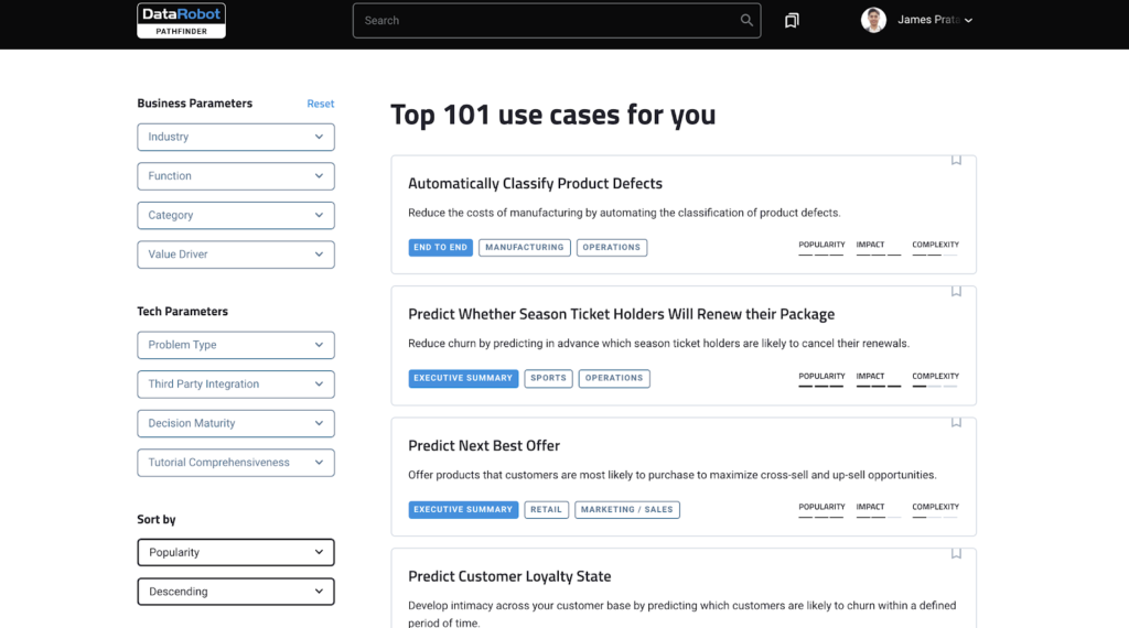
Enter DataRobot Pathfinder, the industry’s leading resource for practical guidance on how to effectively implement AI. Pathfinder is an online library of more than 100 use cases dedicated to helping you discover relevant use cases and understanding how they can be deployed within your organization. These use cases include agnostic applications of AI, such as forecasting demand, scoring new leads, and reducing customer churn. They also include industry-specific applications of AI, such as reducing hospital readmissions, predicting insurance claims’ severity, and preventing anti-money laundering. 

Pathfinder eliminates the noise to show you what you should prioritize in your roadmap. The tool is also developed around a proven technical and business framework to show how you can implement AI. By familiarizing yourself with this framework, you can understand how to apply AI to even more unique problems that your organization faces. 

With its combination of actionable use cases and applicable best practices, Pathfinder helps you expand your adoption of AI. The tool not only helps data scientists uncover more efficient ways to build and deploy models, but also shows business executives and analysts how they can embed predictions into their decision processes. The content shown on Pathfinder is driven by the collective knowledge of more than 35 of DataRobot’s data scientists, and compiles the knowledge these data scientists have accumulated through decades of academic and industry experience. 

Explore Pathfinder

Discover Use Cases

Pathfinder is home to 100+ use cases across more than ten industries. Our data scientists have curated the use cases on Pathfinder to ensure that they are not only relevant but also representative of their industries. DataRobot does not share customer data, personal data, or sensitive use cases on Pathfinder. 

You can benefit from Pathfinder by discovering use cases which your organization may not have considered before. You can filter the use cases based on their business and technical parameters. This includes the ability to filter by industry, problem type (i.e., regression, classification, time series), and value driver, which helps you find use cases that align with high-level business objectives, such as increasing revenue, decreasing costs, and improving customer experience. 

The tabs displaying each use case are designed for you to intuitively explore and identify relevant use cases, which can be sorted based on their popularity, impact, and complexity. While these are broad generalizations that need to be followed up by a deeper analysis of your organization’s unique position, they can give you a quick, high-level overview of which use cases may fit with your organization’s current data science maturity. For instance, organizations only beginning to implement AI should select low-hanging fruits, such as use cases that are high in impact but low in complexity. 

Understand Use Cases

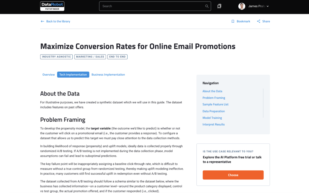
Pathfinder’s use cases are currently segmented by Executive Summary and End-to-End. While Executive Summary only offers high-level overviews of a use case, End-to-End provides detailed guides on how a use case can be implemented from both technical and business perspectives. Pathfinder has more than 30 End-to-End use cases, and more are being released on a regular basis. 

With Pathfinder’s End-to-End guides, you can understand how to build models for specific use cases and deploy their predictions into your decision environments. 

On the technical side, Pathfinder helps you frame use cases into data science problems and reveals the features you will need to train your models. The tool also shows step-by-step tutorials on how to interpret and evaluate models using the DataRobot AI platform. 

On the business side, decision environments are the methods by which predictions will ultimately be used for business decision-making. Pathfinder will guide you towards understanding which stakeholders should consume the predictions, how they will consume the predictions, and what actionable decisions they can make to impact real-world business processes. 

Share Use Cases 

Once you have explored Pathfinder and identified use cases relevant to your organization, you can shortlist these use cases by bookmarking them. These bookmarks will appear on your personal AI roadmap and be saved for future viewing. You can easily share your roadmap with colleagues, who can then curate your list and select specific use cases to add to their own roadmap. 

Find Your Path to AI Success Today 

Pathfinder is available for free to the general public. Whether you are just starting your journey or are years into deploying use cases, Pathfinder will help you uncover new opportunities to expand your AI footprint. We are thrilled to be a small part of your efforts to generate greater value for your organization through automation and optimization. 

Use Case Library

Find your path to AI success with Pathfinder

100+ practical use cases at your fingertips

  Explore

The post Find Your Path to AI Success with DataRobot Pathfinder appeared first on DataRobot.

from Blog – DataRobot https://ift.tt/3isOMkf
via Gabe's MusingsGabe's Musings

How To Compare Two Dataframes with Pandas compare?

Sometimes you may have two similar dataframes and would like to know exactly what those differences are between the two data frames. Starting from Pandas 1.1.0 version, Pandas has a new function compare() that lets you compare two data frames or Series and identify the differences between them and nicely tabulate them.

In this post let us see a simple example of Pandas compare function on two similar data frames and summarize the differences.
Let us load Pandas and Numpy.

import pandas as pd
import numpy as np

Let us check Pandas version and make sure we have Pandas version 1.1.0 and above. Otherwise make sure to install the latest version of Pandas using conda/pip install.

pd.__version__
'1.1.0'

We will first create a toy dataframe with three columns and four rows.

# create dataframe
df1 = pd.DataFrame(
    {
       "col1": ["a", "v", "x", "y"],
       "col2": [1.0, 2.0, 3.0, np.nan],
       "col3": [7.0, 8.0, 9.0, 3.0]
     },
    columns=["col1", "col2", "col3"],
)

And this is how our data looks like.

df1

      col1      col2    col3
0       a       1.0     7.0
1       v       2.0     8.0
2       x       3.0     9.0
3       y       NaN     3.0

Let us create second dataframe by copying the first dataframe and making two changes. In this example, we change the values of first row in first column and second row in second column.

# create a copy of dataframe
df2 = df1.copy()
# change the values of few elements
df2.loc[0, 'col1'] = 'zz'
df2.loc[1, 'col2'] = '10'

If we compare it to the first data frame, it differs in just two places in the first two rows.

df2

     col1       col2    col3
0       zz      1       7.0
1       v       10      8.0
2       x       3       9.0
3       y       NaN     3.0

Let us use Pandas compare() function to summarize the differences between the two dataframes. Pandas compare() function outputs the columns and elements that is different between the dataframes. “self” label in the result correspond to the dataframe that we compare and “other” label corresponds to the dataframe that we compare to.

By default, if two corresponding values are equal, they will be shown as NaN. Furthermore, if all values in an entire row / column, the row / column will be omitted from the result. The remaining differences will be aligned on columns.

df1.compare(df2)

            col1        col2
       self     other   self    other
0       a       zz      NaN     NaN
1       NaN     NaN     2.0     10

We can also change how Pandas compare display result. Here with align_axis=”rows” or align_axis=0, Pandas compare() function displays self and other in separate rows.

df1.compare(df2, align_axis='rows')

        col1     col2
0       self    a       NaN
      other     zz      NaN
1       self    NaN     2
      other     NaN     10

The post How To Compare Two Dataframes with Pandas compare? appeared first on Python and R Tips.

from Python and R Tips https://ift.tt/2BOIxHI
via Gabe's MusingsGabe's Musings

SVD: One Matrix Decomposition to Rule Them All

One of the nice things about twitter, when you follow awesome people, is that you will come across tweets that will just blow your mind. Last week is just one such week with some fantastic and funniest tweetorials.

One of the tweetorials was from Prof. Daniela Witten for @WomenInStat. And it starts like this and beautifully explains why Singular Value Decomposition – SVD in short, is the one matrix decomposition that rules over all the others.

So yesterday I asked you all what you wanted to hear about from me this week, and one answer stood out from all the others: the SINGULAR VALUE DECOMPOSITION (SVD).https://t.co/9Nyqp2Kr9k

1/

— Women in Statistics and Data Science (@WomenInStat) July 21, 2020

Being always in the #teamSVD camp, here is a blog post that tries to unpack some of the tweets with real data example using the awesome Penguins data.

Before we jump in to SVD, let us load tidyverse, the suit of R packages.

library("tidyverse")
theme_set(theme_bw(16))

We will use the Palmer Penguins data collated by Allison Horst directly from cmdlinetips.com‘s github page.

p2data <- "https://raw.githubusercontent.com/cmdlinetips/data/master/palmer_penguins.csv"

penguins_df <- read_csv(p2data)
penguins_df %>% head()
## # A tibble: 6 x 7
##   species island bill_length_mm bill_depth_mm flipper_length_… body_mass_g sex  
##   <chr>   <chr>           <dbl>         <dbl>            <dbl>       <dbl> <chr>
## 1 Adelie  Torge…           39.1          18.7              181        3750 male 
## 2 Adelie  Torge…           39.5          17.4              186        3800 fema…
## 3 Adelie  Torge…           40.3          18                195        3250 fema…
## 4 Adelie  Torge…           NA            NA                 NA          NA <NA> 
## 5 Adelie  Torge…           36.7          19.3              193        3450 fema…
## 6 Adelie  Torge…           39.3          20.6              190        3650 male

Let us separate the numerical data part of the penguins data from the columns with penguin information.

penguins_meta <- penguins_df %>% 
  drop_na() %>% 
  select_if(is.character)
 
penguins_meta %>% head()
## # A tibble: 6 x 3
##   species island    sex   
##   <chr>   <chr>     <chr> 
## 1 Adelie  Torgersen male  
## 2 Adelie  Torgersen female
## 3 Adelie  Torgersen female
## 4 Adelie  Torgersen female
## 5 Adelie  Torgersen male  
## 6 Adelie  Torgersen female

We store the numerical variables describing penguins in a new variable and use it to do SVD.

penguins <- penguins_df %>% 
  drop_na() %>% 
  select_if(is.numeric)
 
penguins %>% head()
## # A tibble: 6 x 4
##   bill_length_mm bill_depth_mm flipper_length_mm body_mass_g
##            <dbl>         <dbl>             <dbl>       <dbl>
## 1           39.1          18.7               181        3750
## 2           39.5          17.4               186        3800
## 3           40.3          18                 195        3250
## 4           36.7          19.3               193        3450
## 5           39.3          20.6               190        3650
## 6           38.9          17.8               181        3625

What is Singular Value Decomposition (SVD)?

First of all, what does the SVD do? You give me an $n \times p$ matrix $X$, and I’ll give you back 3 matrices $U$, $D$, $V$. Without loss of generality let’s assume that $n \geq p$. Then $U$ is an $n \times p$ matrix, and $D$ and $V$ have dimension $p \times p$.

7/

— Women in Statistics and Data Science (@WomenInStat) July 21, 2020

We can use svd() function in R to do SVD. We provide the data matrix as input to svd() function.

# perform SVD using svd()
penguins_svd <- svd(penguins)

What happens when we apply svd() to a data matrix?

$U$, $D$, $V$ “decompose” the matrix $X$ because $X=UDV^T$. Simple as that. But, what makes this decomposition special (and unique) is the particular set of properties of $U$, $D$, and $V$.

8/ pic.twitter.com/TYG4enUMhE

— Women in Statistics and Data Science (@WomenInStat) July 21, 2020

In R, we get a list of three objects corresponding to matrix decomposition, singular values d, and singular vectors u and v from svd() function.

str(penguins_svd)
## List of 3
##  $ d: num [1:4] 78250.5 499.9 74 41.8
##  $ u: num [1:333, 1:4] -0.048 -0.0486 -0.0416 -0.0442 -0.0467 ...
##  $ v: num [1:4, 1:4] -0.01022 -0.00389 -0.04657 -0.99886 0.1985 ...

Let us take a look at the singular values and vectors and understand their properties. For the sake of simplicity, let us give a simple name to singular values and vectors.

The sigular vector U is a matrix of dimension 333 x 4, the same dimension as our data.

U <- penguins_svd$u
U %>% dim()
## [1] 333   4

And it looks like this.

U %>% head()

##             [,1]       [,2]        [,3]        [,4]
## [1,] -0.04798188 0.01338848 0.004108109  0.07663240
## [2,] -0.04862309 0.01809574 0.014438916  0.03365464
## [3,] -0.04160792 0.08855716 0.025312973 -0.01876370
## [4,] -0.04415929 0.06451464 0.067224723  0.03968621
## [5,] -0.04671088 0.04099607 0.024614580  0.08738297
## [6,] -0.04638621 0.02499507 0.006737752  0.04717352

Similarly, the singular vectors V is of the dimension 4 x 4.

V <- penguins_svd$v

And the singular vectors V looks like these.

V %>% head()
##              [,1]        [,2]         [,3]         [,4]
## [1,] -0.010218185  0.19849831 -0.975661291 -0.092623187
## [2,] -0.003891394  0.14068499 -0.065122188  0.987902673
## [3,] -0.046569777  0.96877576  0.209389404 -0.124341735
## [4,] -0.998855196 -0.04774608  0.000472226  0.002896004

And finally, the singular values D we get is a vector of length 4.

D <- penguins_svd$d
D
## [1] 78250.54165   499.88402    74.04578    41.84098

What is special about these singular matrices?

The singular matrices U and V are orthogonal. What this means is if you multiply U with transpose of U, you will get an identity matrix with ones along diagonal and zeros elsewhere. This is true for the singular matrix V as well.

svd_orthogonal_matrix

Let us verify the orthogonal properties of the singular matrices from the penguin data.

t(U) %*% U

We can see that diagonal elements are ones and off diagonal elements pretty close to zero.

##              [,1]         [,2]          [,3]          [,4]
## [1,] 1.000000e+00 2.038300e-16  3.816392e-17  6.126555e-16
## [2,] 2.038300e-16 1.000000e+00  2.289835e-16  2.167862e-16
## [3,] 3.816392e-17 2.289835e-16  1.000000e+00 -1.156844e-16
## [4,] 6.126555e-16 2.167862e-16 -1.156844e-16  1.000000e+00

And this is true of the singular matrix V as well.

t(V) %*% V
##               [,1]          [,2]          [,3]          [,4]
## [1,]  1.000000e+00 -4.857226e-17  1.919038e-17 -3.473784e-16
## [2,] -4.857226e-17  1.000000e+00  2.058629e-17  5.583641e-18
## [3,]  1.919038e-17  2.058629e-17  1.000000e+00 -1.406308e-17
## [4,] -3.473784e-16  5.583641e-18 -1.406308e-17  1.000000e+00

Also, this is true if you change the order of multiplication as well.

V %*% t(V)
##               [,1]         [,2]          [,3]          [,4]
## [1,]  1.000000e+00 5.551115e-17  2.255141e-17 -6.179952e-18
## [2,]  5.551115e-17 1.000000e+00  8.326673e-17  3.486794e-16
## [3,]  2.255141e-17 8.326673e-17  1.000000e+00 -1.534146e-17
## [4,] -6.179952e-18 3.486794e-16 -1.534146e-17  1.000000e+00

Another special property of the singular vectors is that orthonormal. What this means is that the squared elements of each column of U sums to 1. And the inner product (dot product) between any pair of columns in U equals to 0. And the inner product between each pair of columns of V equals 0. The same is true for V columns as well.

svd_singular_vectors

Let us first check if the squared elements of each column equals 1 for U and V.

colSums(U^2)
## [1] 1 1 1 1

colSums(V^2)
## [1] 1 1 1 1

We see that the sum of squares for each columns of U and V is 1.

Now let us check if the column vectors are orthogonal, i.e. does the inner product of a pair U columns (and also V columns) equals to zero.

We see that the column vectors of U and V are orthogonal.

sum(V[,1]*V[,4])
## [1] -3.474868e-16

sum(U[,1]*U[,2])
## [1] 1.715343e-16

Since both the properties “orthogonal” and “normality” hold true for U and V, we say that the singular vectors are orthonormal.

Reconstructing Original data with a few singular vectors

One of the common applications of SVD is in data compression or dimensionality reduction. The original data matrix with bigger dimension can be approximated with one or few singular vectors.

SVD_rank_1_approximation

Let us reconstruct an approximate version of the original data using one column vector from U and V and the first singular value. We get rank-1 approximation of the data.

D[1] * (U[,1] %*% t(V[,1])) %>% head()
##          [,1]     [,2]     [,3]     [,4]
## [1,] 38.36528 14.61066 174.8513 3750.310
## [2,] 38.87798 14.80591 177.1879 3800.427
## [3,] 33.26880 12.66977 151.6239 3252.115
## [4,] 35.30882 13.44667 160.9213 3451.533
## [5,] 37.34901 14.22364 170.2196 3650.967
## [6,] 37.08941 14.12477 169.0365 3625.591

Let us check the top few rows from rank-1 approximate data with the original data. And we can see that, rank-1 approximation is pretty close to original data.

penguins %>% head()
## # A tibble: 6 x 4
##   bill_length_mm bill_depth_mm flipper_length_mm body_mass_g
##            <dbl>         <dbl>             <dbl>       <dbl>
## 1           39.1          18.7               181        3750
## 2           39.5          17.4               186        3800
## 3           40.3          18                 195        3250
## 4           36.7          19.3               193        3450
## 5           39.3          20.6               190        3650
## 6           38.9          17.8               181        3625

We can improve our ability to reconstruct by using more singular vectors.

SVD_rank_2_approximation

In this case let us compute rank-2 approximation of data matrix using the first column singular vectors and singular values.

((D[1] * (U[,1] %*% t(V[,1])))+ (D[2] * (U[,2] %*% t(V[,2]))))  %>% head()

##          [,1]     [,2]     [,3]     [,4]
## [1,] 39.69377 15.55222 181.3350 3749.991
## [2,] 40.67355 16.07852 185.9512 3799.995
## [3,] 42.05598 18.89765 194.5099 3250.001
## [4,] 41.71036 17.98374 192.1642 3449.993
## [5,] 41.41689 17.10673 190.0730 3649.989
## [6,] 39.56958 15.88258 181.1410 3624.994

When we compare this to original penguins data, we can see that it is a very good approximation.

Computing PCA from SVD

Principal component analysis is just a special case of SVD. Applying SVD on the data matrix whose columns are centered, is doing PCA. Columns of V are PC loading vectors. Columns of U are PC score vectors.

PCA is a special case of SVD

Let us allply SVD on mean centered Penguins data. By mean centering, we are putting all the variables/columns in the data on the same scale. Therefore a single variable with a huge range would not dominate.

# mean centering the columns
data4pca <- apply(penguins,2,function(x){x-mean(x)})
# apply SVD
pca_by_svd <- svd(data4pca)
# get a peek at V singular vectors
pca_by_svd$v %>% head()
##              [,1]        [,2]        [,3]          [,4]
## [1,]  0.004003162 -0.31927773 -0.94126475 -0.1098470736
## [2,] -0.001154327  0.08684753 -0.14449479  0.9856862728
## [3,]  0.015194547 -0.94354238  0.30518986  0.1278908060
## [4,]  0.999875876  0.01571702 -0.00103611 -0.0003657482

Let us also apply PCA on Penguins data using prcomp() function. Notice that rotation matrix from PCA is the same as V singular vectors from SVD on mean centered data.

pca_obj <- prcomp(penguins)
pca_obj$rotation %>% head()
##                            PC1         PC2         PC3           PC4
## bill_length_mm     0.004003162 -0.31927773 -0.94126475 -0.1098470736
## bill_depth_mm     -0.001154327  0.08684753 -0.14449479  0.9856862728
## flipper_length_mm  0.015194547 -0.94354238  0.30518986  0.1278908060
## body_mass_g        0.999875876  0.01571702 -0.00103611 -0.0003657482

t(as.matrix(penguins)) %*% as.matrix(penguins)
##                   bill_length_mm bill_depth_mm flipper_length_mm body_mass_g
## bill_length_mm          654405.7     250640.99           2960705    62493450
## bill_depth_mm           250641.0      99400.11           1143413    23798630
## flipper_length_mm      2960705.0    1143412.60          13514330   284815600
## body_mass_g           62493450.0   23798630.00         284815600  6109136250

SVD from Scratch: A Pair of Singular Vectors at a time

What is all the more interesting is writing a function from scratch to perform SVD is relatively easy. We can write a function that computes a pair of U and V using an iterative approach. Idea is to compute the first U and V singular vectors from the data iteratively and then remove the rank-1 approximation from the data and apply the approach to compute the second U and V singular vectors.

Implementing SVD from Scratch

Here is an R function that computes the first singular vectors of SVD from scrtach

svd_from_scratch <- function(data){
  # initialize u and v with random numbers
  u <- rnorm(nrow(data))
  v <- rnorm(ncol(data))
  for (iter in 1:500){
    u <- data %*% v
    u <-  u/sqrt(sum(u^2))
    v <- t(data) %*% u
    v <- v / sqrt(sum(v^2))
    }
  return(list(u=u,v=v))
}

svdx <- svd_from_scratch(as.matrix(penguins))

cor(U[,1],svdx$u)
##      [,1]
## [1,]   -1
cor(V[,1],svdx$v)
##      [,1]
## [1,]   -1

If you love the tweetorial from Prof. Daniela Witten, you would love the “An Introduction to Statistical Learning with Applications in R” co-authored by Prof. Witten. And it is freely available online.

And can’t wait to get my hands on the Second Edition of the book

If you like #islr first edition then you will love ? ? our second edition… coming soon!! https://t.co/9w1DSYJAgH

— Daniela Witten (@daniela_witten) May 16, 2020

The post SVD: One Matrix Decomposition to Rule Them All appeared first on Python and R Tips.

from Python and R Tips https://ift.tt/30Qw8LR
via Gabe's MusingsGabe's Musings

dplyr mutate(): Create New Variables with mutate

Create new column with dplyr mutate

dplyr, R package part of tidyverse suite of packages, provides a great set of tools to manipulate datasets in the tabular form. dplyr has a set of core functions for “data munging”,including select(), mutate(), filter(), summarise(), and arrange().

And in this tidyverse tutorial, a part of tidyverse 101 series, we will learn how to use dplyr’s mutate() function. With dplyr’s mutate() function one can create a new variable/column in the data frame. Here we will use dplyr’s mutate() function to create one variable first and multiple variables at the same time.

library("tidyverse")

We will use the fantastic Penguins dataset to illustrate the three ways to see data in a dataframe. Let us load the data from cmdlinetips.com‘ github page.

path2data <- "https://raw.githubusercontent.com/cmdlinetips/data/master/palmer_penguins.csv"
penguins<- readr::read_csv(path2data)

We can see that our data frame contains multiple variables that are mesaured in milli-meter (mm) and a variable measured in gram (g).

## Parsed with column specification:
## cols(
##   species = col_character(),
##   island = col_character(),
##   bill_length_mm = col_double(),
##   bill_depth_mm = col_double(),
##   flipper_length_mm = col_double(),
##   body_mass_g = col_double(),
##   sex = col_character()
## )

How To Create A New Variable with mutate() in dplyr?

Let us create a single new column using dplyr’s mutate(). We will use an existing column to create the new column or variable.

Our new variable is body_mass in kg and we will compute it from existing variable body_mass_g. To create the new variable, we start with the data frame with the pipe operator and use mutate() function. Inside mutate() function, we specify the name of the new variable we are creating and how exactly we are creating. In this example, we create the new variable body_mass_kg by dividing an existing variable body_mass_g by 1000.

penguins %>% 
  mutate(body_mass_kg = body_mass_g/1000)

We get a data frame with the new column as result. The new variable that we created will be added as the last column. the

## # A tibble: 344 x 8
##    species island bill_length_mm bill_depth_mm flipper_length_… body_mass_g
##    <chr>   <chr>           <dbl>         <dbl>            <dbl>       <dbl>
##  1 Adelie  Torge…           39.1          18.7              181        3750
##  2 Adelie  Torge…           39.5          17.4              186        3800
##  3 Adelie  Torge…           40.3          18                195        3250
##  4 Adelie  Torge…           NA            NA                 NA          NA
##  5 Adelie  Torge…           36.7          19.3              193        3450
##  6 Adelie  Torge…           39.3          20.6              190        3650
##  7 Adelie  Torge…           38.9          17.8              181        3625
##  8 Adelie  Torge…           39.2          19.6              195        4675
##  9 Adelie  Torge…           34.1          18.1              193        3475
## 10 Adelie  Torge…           42            20.2              190        4250
## # … with 334 more rows, and 2 more variables: sex <chr>, body_mass_kg <dbl>

Note that creating a new column with mutate() does not change the original dataframe. We get a new dataframe as a tibble.

How to Create two variables with mutate?

We can create two or more new variables using a single mutate function. For example, to create two new columns, we use mutate() fucntions with new variables separated by comma.

In this example below we create two new variables using existing variables.

penguins %>% 
  mutate(body_mass_kg= body_mass_g/1000,
         flipper_length_m = flipper_length_mm/1000)

## # A tibble: 344 x 9
##    species island bill_length_mm bill_depth_mm flipper_length_… body_mass_g
##    <chr>   <chr>           <dbl>         <dbl>            <dbl>       <dbl>
##  1 Adelie  Torge…           39.1          18.7              181        3750
##  2 Adelie  Torge…           39.5          17.4              186        3800
##  3 Adelie  Torge…           40.3          18                195        3250
##  4 Adelie  Torge…           NA            NA                 NA          NA
##  5 Adelie  Torge…           36.7          19.3              193        3450
##  6 Adelie  Torge…           39.3          20.6              190        3650
##  7 Adelie  Torge…           38.9          17.8              181        3625
##  8 Adelie  Torge…           39.2          19.6              195        4675
##  9 Adelie  Torge…           34.1          18.1              193        3475
## 10 Adelie  Torge…           42            20.2              190        4250
## # … with 334 more rows, and 3 more variables: sex <chr>, body_mass_kg <dbl>,
## #   flipper_length_m <dbl>

How To Create a Fresh New Column with dplyr’s mutate

In the above examples, we create one or more new columns from an existing columns. We can use mutate() function to create without using existing column as well.

In this example, we use dplyr’s mutate() function to create new column using row number.

penguins %>% 
   mutate(ID=row_number())

This creates ID column at the end of the dataframe.

## # A tibble: 344 x 8
##    species island bill_length_mm bill_depth_mm flipper_length_… body_mass_g
##    <chr>   <chr>           <dbl>         <dbl>            <dbl>       <dbl>
##  1 Adelie  Torge…           39.1          18.7              181        3750
##  2 Adelie  Torge…           39.5          17.4              186        3800
##  3 Adelie  Torge…           40.3          18                195        3250
##  4 Adelie  Torge…           NA            NA                 NA          NA
##  5 Adelie  Torge…           36.7          19.3              193        3450
##  6 Adelie  Torge…           39.3          20.6              190        3650
##  7 Adelie  Torge…           38.9          17.8              181        3625
##  8 Adelie  Torge…           39.2          19.6              195        4675
##  9 Adelie  Torge…           34.1          18.1              193        3475
## 10 Adelie  Torge…           42            20.2              190        4250
## # … with 334 more rows, and 2 more variables: sex <chr>, ID <int>

How To Overwrite an Existing Column with dplyr’s mutate

We can also use dplyr’s mutate() function to overwrite an existing column. In the example below, we use mutate() function to overwrite the existing “species” variable.

penguins %>%
  mutate(species= stringr::str_to_upper(species))

We use str_to_upper() function from stringr package to convert the character variable to uppercase variable. Note the values of the first column species is all in upper case now.

## # A tibble: 344 x 7
##    species island bill_length_mm bill_depth_mm flipper_length_… body_mass_g
##    <chr>   <chr>           <dbl>         <dbl>            <dbl>       <dbl>
##  1 ADELIE  Torge…           39.1          18.7              181        3750
##  2 ADELIE  Torge…           39.5          17.4              186        3800
##  3 ADELIE  Torge…           40.3          18                195        3250
##  4 ADELIE  Torge…           NA            NA                 NA          NA
##  5 ADELIE  Torge…           36.7          19.3              193        3450
##  6 ADELIE  Torge…           39.3          20.6              190        3650
##  7 ADELIE  Torge…           38.9          17.8              181        3625
##  8 ADELIE  Torge…           39.2          19.6              195        4675
##  9 ADELIE  Torge…           34.1          18.1              193        3475
## 10 ADELIE  Torge…           42            20.2              190        4250
## # … with 334 more rows, and 1 more variable: sex <chr>

The post dplyr mutate(): Create New Variables with mutate appeared first on Python and R Tips.

from Python and R Tips https://ift.tt/3fKaDCC
via Gabe's MusingsGabe's Musings

dplyr select(): Select one or more variables from a dataframe

dplyr select(): How to Select Columns?

dplyr, R package part of tidyverse, provides a great set of tools to manipulate datasets in the tabular form. dplyr has a set of core functions for “data munging”. Here is the list of core functions from dplyr

• select() picks variables based on their names.
• mutate() adds new variables that are functions of existing variables
• filter() picks cases based on their values.
• summarise() reduces multiple values down to a single summary.
• arrange() changes the ordering of the rows.

And in this tidyverse tutorial, we will learn how to use dplyr’s select() function to pick/select variables/columns from a dataframe by their names. First we will start with how to select a single variable by its name and then we will see examples of selecting multiple variables/columns by their names.

Let us get started by loading tidyverse.

library("tidyverse")

For our tutorial on tidyverse, we will use the Palmer Penguins dataset collated by Allison Horst to illustrate how to use dplyr’s select() function to select variables by their names. Let us load the data from cmdlinetips.com’ github page.

path2data <- "https://raw.githubusercontent.com/cmdlinetips/data/master/palmer_penguins.csv"
penguins<- readr::read_csv(path2data)

We can take a glimpse of the data using glimpse() function.

glimpse(penguins)

Rows: 344
Columns: 7
$ species           <chr> "Adelie", "Adelie", "Adelie", "Adelie", "Adelie", "Adelie", …
$ island            <chr> "Torgersen", "Torgersen", "Torgersen", "Torgersen", "Torgers…
$ bill_length_mm    <dbl> 39.1, 39.5, 40.3, NA, 36.7, 39.3, 38.9, 39.2, 34.1, 42.0, 37…
$ bill_depth_mm     <dbl> 18.7, 17.4, 18.0, NA, 19.3, 20.6, 17.8, 19.6, 18.1, 20.2, 17…
$ flipper_length_mm <dbl> 181, 186, 195, NA, 193, 190, 181, 195, 193, 190, 186, 180, 1…
$ body_mass_g       <dbl> 3750, 3800, 3250, NA, 3450, 3650, 3625, 4675, 3475, 4250, 33…
$ sex               <chr> "male", "female", "female", NA, "female", "male", "female", …

How To Select A Variable by name with dplyr select()?

We can select a variable from a data frame using select() function in two ways. One way is to specify the dataframe name and the variable/column name we want to select as arguments to select() function in dplyr.

In this example below, we select species column from penguins data frame. One big advantage with dplyr/tidyverse is the ability to specify the variable names without quotes.

select(penguins, species)

The result is a type of dataframe called tibble with just one column we selected.

## # A tibble: 344 x 1
##    species
##    <chr>  
##  1 Adelie 
##  2 Adelie 
##  3 Adelie 
##  4 Adelie 
##  5 Adelie 
##  6 Adelie 
##  7 Adelie 
##  8 Adelie 
##  9 Adelie 
## 10 Adelie 
## # … with 334 more rows

The second way to select a column from a dataframe is to use the pipe operator %>% available as part of tidyverse.

Here we first specify the name of the dataframe we want to work with and use the pipe %>% operator followed by select function with the column name we want to select.

penguins %>% select(species)

We get the same data frame as tibble with a single column as before.

## # A tibble: 344 x 1
##    species
##    <chr>  
##  1 Adelie 
##  2 Adelie 
##  3 Adelie 
##  4 Adelie 
##  5 Adelie 
##  6 Adelie 
##  7 Adelie 
##  8 Adelie 
##  9 Adelie 
## 10 Adelie 
## # … with 334 more rows

The use of pipe operator can be extremely useful when we further down stream operations after selecting. Therefore, in the examples below we will the pipe operator way to select multiple columns

How To Select Two Variables by name with dplyr select()?

If we want to select two variables/columns from a dataframe, we specify the two names as arguments. In this example we select species and island columns from the dataframe using the pipe operator.

penguins %>% select(species, island)

## # A tibble: 344 x 2
##    species island   
##    <chr>   <chr>    
##  1 Adelie  Torgersen
##  2 Adelie  Torgersen
##  3 Adelie  Torgersen
##  4 Adelie  Torgersen
##  5 Adelie  Torgersen
##  6 Adelie  Torgersen
##  7 Adelie  Torgersen
##  8 Adelie  Torgersen
##  9 Adelie  Torgersen
## 10 Adelie  Torgersen
## # … with 334 more rows

How To Select Multiple Variables by name with dplyr select()?

Similarly, if we have more variables to select, we specify the names as argument to select() function in dplyr as shown below.

5.3 Select Multiple Columns
penguins %>% select(species, body_mass_g, sex)
## # A tibble: 344 x 3
##    species body_mass_g sex   
##    <chr>         <dbl> <chr> 
##  1 Adelie         3750 male  
##  2 Adelie         3800 female
##  3 Adelie         3250 female
##  4 Adelie           NA <NA>  
##  5 Adelie         3450 female
##  6 Adelie         3650 male  
##  7 Adelie         3625 female
##  8 Adelie         4675 male  
##  9 Adelie         3475 <NA>  
## 10 Adelie         4250 <NA>  
## # … with 334 more rows

The post dplyr select(): Select one or more variables from a dataframe appeared first on Python and R Tips.

from Python and R Tips https://ift.tt/2CjWIoG
via Gabe's MusingsGabe's Musings

How To Change Pandas Column Names to Lower Case?

Cleaning up the column names of a dataframe often can save a lot of head aches while doing data analysis. In this post, we will learn how to change column names of a Pandas dataframe to lower case. And then we will do additional clean up of columns and see how to remove empty spaces around column names.

Let us load Pandas and scipy.stats.

import pandas as pd
from scipy.stats import poisson

We will create a toy dataframe with three columns. We will first name the dataframe’s columns with upper cases.

c1= poisson.rvs(mu=10, size=5)
c2= poisson.rvs(mu=15, size=5)
c3= poisson.rvs(mu=20, size=5)
df=pd.DataFrame({"COLUMN1":c1,
                 "COLUMN2":c2,
                 "COLUMN3":c3})

Our data frame’s column names starts with uppercase.

df.head()
COLUMN1 COLUMN2 COLUMN3
0       16      12      16
1       12      14      11
2       15      15      23
3       8       14      24
4       11      15      32

How To Convert Pandas Column Names to lowercase?

We can convert the names into lower case using Pandas’ str.lower() function. We first take the column names and convert it to lower case.

And then rename the Pandas columns using the lowercase names. Now our dataframe’s names are all in lower case.

# rename Pandas columns to lower case
df.columns= df.columns.str.lower()
df.columns
Index(['column1', 'column2', 'column3'], dtype='object')

Cleaning up Pandas Column Names

In addition to upper cases, sometimes column names can have both leading and trailing empty spaces. Let us create a toy dataframe with column names having trailing spaces.

df=pd.DataFrame({" C1 ":c1,
                 "C2":c2,
                 "C3 ":c3})

By inspecting column names we can see the spaces.

df.columns
Index([' C1 ', 'C2', 'C3 '], dtype='object')

We can use str.strip() function Pandas to strip the leading and trailing white spaces. Here we also convert the column names into lower cases using str.lower() as before.

# Column names: remove white spaces and convert to lower case
df.columns= df.columns.str.strip().str.lower()
df.columns

Index(['c1', 'c2', 'c3'], dtype='object')

We use Pandas chaining operation to do both and re-assign the cleaned column names.

df

c1      c2      c3
0       16      12      16
1       12      14      11
2       15      15      23
3       8       14      24
4       11      15      32

The post How To Change Pandas Column Names to Lower Case? appeared first on Python and R Tips.

from Python and R Tips https://ift.tt/38ZedGG
via Gabe's MusingsGabe's Musings

Pandas Groupby and Sum

A common step in data analysis is to group the data by a variable and compute some summary statistics each subgroup of data. For example, one might be interested in mean, median values, or total sum per group. In this post, we will see an example of how to use groupby() function in Pandas to group a dataframe into multiple smaller dataframes and compute total/sum on another variable.

Let us load the libraries we need.

import pandas as pd
import numpy as np

We will use gapminder dataset to learn groupby() and sum() functions to summarise data at a group level.

p2data = "https://raw.githubusercontent.com/cmdlinetips/data/master/gapminder-FiveYearData.csv"
gapminder=pd.read_csv(p2data)
gapminder.head()

Let us first subset the data for the sake of simplicity. Here we filter data for year values 2007 using Pandas filter() function.

df= gapminder.query("year==2007")
df.head()

With the data corresponding to the year 2007, let us compute total population in each continent. In order to do that, we first need to use groupby() to group the data corresponding to each continent.

df.groupby(["continent"])
<pandas.core.groupby.generic.DataFrameGroupBy object at 0x1a19c9c850>

From the grouped object, let us select our variable of interest. Since we are interested in computing total population, we select “pop”

df.groupby(["continent"])['pop']
<pandas.core.groupby.generic.SeriesGroupBy object at 0x1a19cc1590>

And chain it with sum() function in Pandas that computes the total population for each continent.

df.groupby(["continent"])['pop'].sum()

Here we have results as Pandas Series with total population for each continent computed by groupby() and sum().

continent
Africa      9.295397e+08
Americas    8.988712e+08
Asia        3.811954e+09
Europe      5.860985e+08
Oceania     2.454995e+07
Name: pop, dtype: float64

This post is part of the series on Pandas 101, a tutorial covering tips and tricks on using Pandas for data munging and analysis.

The post Pandas Groupby and Sum appeared first on Python and R Tips.

from Python and R Tips https://ift.tt/2ZjmdPm
via Gabe's MusingsGabe's Musings